Previous
Bayesian Network
Contents
Table of Contents
Next
ANN

7.4.2. Gaussian Processes

Gaussian processes may not be at the center of the current machine learning hype, but they are still used at the forefront of research. For instance, they were employed to automatically tune the MCTS hyperparameters for AlphaGo Zero. This type of nonparametric Bayesian algorithm can be very easy to use while providing rich modeling capacity and uncertainty estimates. However, the algorithm is not that easy to grasp, especially if you are new to nonparametric models. This section is proposed to present a more visual and intuitive introduction to Gaussian processes without totally abandoning the theory.

Introduction to Gaussian Process

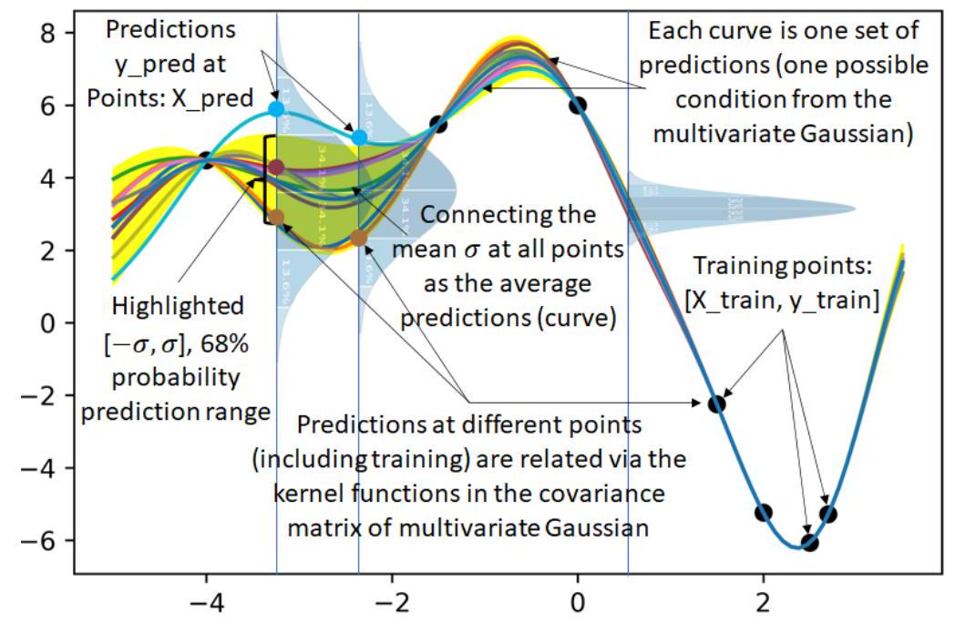
A Gaussian Process (GP) is a powerful model that can be used to represent a "distribution (Gaussian) of functions" [65]. In a 2D regression problem, this distribution of functions can be visualized as a Gaussian distribution of curves, as shown in Fig. 7.5. That is, after the "training process" is finished, we would obtain an infinite number of fitting curves that are associated with different probabilities at a finite number of data points. Among them, we have a curve with the highest probability, i.e., the mean curve or the curve connecting all the mean values at the data points. We can also obtain confidence intervals, e.g., a range where a certain percentage of curves will fall in.
Figure 7.5: Conceptual illustration of Gaussian Process
Usually, we do the regression at a finite number of given data points (training and testing). In GP, the prediction or the label of each data point can be viewed as a random variable that obeys the Gaussian distribution. Accordingly, all the random variables corresponding to all the points form a multivariate Gaussian distribution, as illustrated in the following equation.
(7.39) [ y 0 y 1 y I ] N ( μ , Σ ¯ ) N ( [ 0 0 0 ] , [ σ 11 σ 12 σ 1 I σ 21 σ 22 σ 2 I σ I 1 σ I 2 σ I I ] ) (7.39) y 0 y 1 y I N ( μ , Σ ¯ ) N 0 0 0 , σ 11 σ 12 σ 1 I σ 21 σ 22 σ 2 I σ I 1 σ I 2 σ I I {:(7.39)[[y_(0)],[y_(1)],[vdots],[y_(I)]]∼N( vec(mu)"," bar(Sigma))∼N([[0],[0],[vdots],[0]],[[sigma_(11),sigma_(12),cdots,sigma_(1I)],[sigma_(21),sigma_(22),cdots,sigma_(2I)],[vdots,vdots,ddots,vdots],[sigma_(I1),sigma_(I2),cdots,sigma_(II)]]):}\left[\begin{array}{c} y_{0} \tag{7.39}\\ y_{1} \\ \vdots \\ y_{I} \end{array}\right] \sim \mathcal{N}(\vec{\mu}, \bar{\Sigma}) \sim \mathcal{N}\left(\left[\begin{array}{c} 0 \\ 0 \\ \vdots \\ 0 \end{array}\right],\left[\begin{array}{cccc} \sigma_{11} & \sigma_{12} & \cdots & \sigma_{1 I} \\ \sigma_{21} & \sigma_{22} & \cdots & \sigma_{2 I} \\ \vdots & \vdots & \ddots & \vdots \\ \sigma_{I 1} & \sigma_{I 2} & \cdots & \sigma_{I I} \end{array}\right]\right)(7.39)[y0y1yI]N(μ,Σ¯)N([000],[σ11σ12σ1Iσ21σ22σ2IσI1σI2σII])
where N ( μ , Σ ¯ ) N ( μ , Σ ¯ ) ∼N( vec(mu), bar(Sigma))\sim \mathcal{N}(\vec{\mu}, \bar{\Sigma})N(μ,Σ¯) means following a Gaussian (normal) distribution characterized by the vector of means μ μ vec(mu)\vec{\mu}μ and a covariance matrix Σ ¯ Σ ¯ bar(Sigma)\bar{\Sigma}Σ¯. Usually, the vector of means is assumed to be a vector of zeros, which is proven adequate to give the 'fitting function' or model enough flexibility. The overall location and trend of the curve are determined by the training data points.
The covariance matrix of the multivariate distribution is determined by a kernel function that defines the covariance coefficient between any two random variables in the matrix. The kernel function or the covariance coefficients calculated with it determine how the values between neighboring points are related to each other - the smoothness of the curve. A typical option for such a kernel function is a squared exponential function.
(7.40) k ( x , x ) = exp [ ( x x ) 2 2 ] (7.40) k x , x = exp x x 2 2 {:(7.40)k(x,x^('))=exp[-((x-x^('))^(2))/(2)]:}\begin{equation*} k\left(x, x^{\prime}\right)=\exp \left[-\frac{\left(x-x^{\prime}\right)^{2}}{2}\right] \tag{7.40} \end{equation*}(7.40)k(x,x)=exp[(xx)22]
Gaussian process is different from many supervised learning methods, because it does not contain the typical training and testing steps, which is called eager learning. By contrast, it is similar to KNN , which is also a nonparametric algorithm, in that both of them belong to lazy learning. In such lazy learning algorithms, there is no obvious training step/stage, and most computing occurs during the testing/prediction. Because of this, this type of machine learning algorithm has a high demand for memory for storing the training data. This difference is very obvious in the implementation of such methods.
Using a 2D regression problem as an example, we have X_train, y_train, and X_test and need to predict y_test. The covariance matrix can then be obtained with these given data and the equations for multivariate Gaussian distributions. With the covariance matrix and a Zero vector of means, we can predict the possible curves consisting of the predicted values of the random variables at the testing data points. With a number of predicted curves, we can get the most possible (mean) curve and confidence intervals. Thus, there are training and testing data but no distinct steps for training and testing.
Also, as described above, the predictions were obtained based on the analytical equations from the training data (X_train, y_train) and X_test directly without assuming any specific math functions for the model. Instead, we only assume the values at all the data points follow a multivariate Gaussian function with a specific kernel function for the covariance coefficients. This is why Gaussian process is usually believed to be a nonparametric machine learning method.

Modeling Functions using Multivariate Gaussian

The key idea behind GP is that a mapping function can be modeled using an infinite dimensional multivariate Gaussian distribution. In other words, every data point in the input space is associated with a random variable, and the joint distribution of these variables is modeled as a multivariate Gaussian. This may not be easy to understand for people who are not familiar with multivariate Gaussian distributions. Let us use a simpler case, i.e., a unit 2D Gaussian, to see what it looks like.
First, let us take a look at a very simple multivariate Gaussian distribution that consists of multiple univariate standard Gaussian distributions. Such a function has a math formulation as follows:
(7.41) [ y 0 y 1 y I ] N ( μ , Σ ¯ ) N ( [ 0 0 0 ] , [ 1 0 0 0 1 0 0 0 1 ] I × I ) (7.41) y 0 y 1 y I N ( μ , Σ ¯ ) N 0 0 0 , 1 0 0 0 1 0 0 0 1 I × I {:(7.41)[[y_(0)],[y_(1)],[vdots],[y_(I)]]∼N( vec(mu)"," bar(Sigma))∼N([[0],[0],[vdots],[0]],[[1,0,dots,0],[0,1,dots,0],[vdots,vdots,ddots,vdots],[0,0,dots,1]]_(I xx I)):}\left[\begin{array}{c} y_{0} \tag{7.41}\\ y_{1} \\ \vdots \\ y_{I} \end{array}\right] \sim \mathcal{N}(\vec{\mu}, \bar{\Sigma}) \sim \mathcal{N}\left(\left[\begin{array}{c} 0 \\ 0 \\ \vdots \\ 0 \end{array}\right],\left[\begin{array}{cccc} 1 & 0 & \ldots & 0 \\ 0 & 1 & \ldots & 0 \\ \vdots & \vdots & \ddots & \vdots \\ 0 & 0 & \ldots & 1 \end{array}\right]_{I \times I}\right)(7.41)[y0y1yI]N(μ,Σ¯)N([000],[100010001]I×I)
Next, let us implement such a function. It is a probability distribution. So, we can sample 10 curves at 20 data points. Accordingly, I I III is 20 in this example.
import numpy as np
              import matplotlib.pyplot as plt
              def plot_unit_gaussian_samples(D):
                p = plt.figure()
              
xs = np.linspace(0, 1, D)
              for color in range(10): # 10 for 10 curves
                ys = np.random.multivariate_normal(np.zeros(D), np.eye(D))
                plt.plot(xs, ys)
                return p
              plot_unit_gaussian_samples(20)
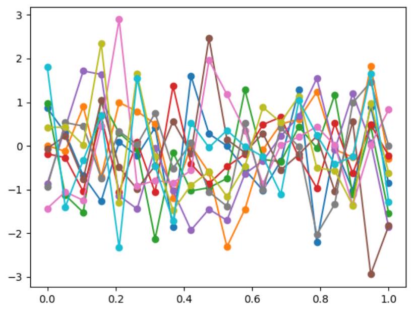
              
As can be seen in Fig. 7.6, 10 curves sampled using this simple multivariate Gaussian distribution are illustrated using different colors. Each predicted value at any of the 20 data points is one sample from a univariate Gaussian distribution. One curve consisting of 20 random variable values was generated at one time. However, the curve is very 'noisy' or 'rough', which is much different from smooth math functions that we typically use for machine learning models. In other words, any two predicted values in each curve are not related. This is caused by the zero non-diagonal values in the covariance matrix, making the 20 predicted values in one curve not different from 20 predicted values from 20 separate standard Gaussian distributions.
Figure 7.6: Samples from a 20D Gaussian without kernel smoothing
In order to obtain smooth functions, we can generate a complicated covariance matrix using a squared exponential kernel equation. This kernel function, together with the Zero array for the mean vector, can be defined using the following code:
def kernel(X1,X2):
                Sigma = np.empty((X1.shape[0],X2.shape[0]))
                for i in range(X1.shape[0]):
                    for j in range(X2.shape[0]):
                        Sigma[i,j] = np.exp(-(X1[i]-X2[j])**2/2)
                return Sigma
              def mean(X):
                Mu = np.zeros(X.shape[0]) #np.mean(X,axis=0)
                return Mu
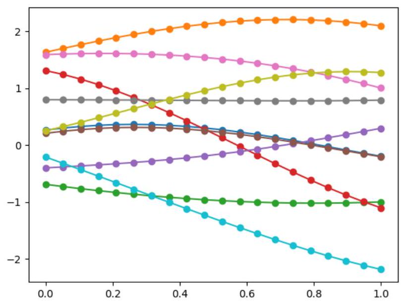
              
So, to get the smoothness we want, we will consider two random variables y i y i y_(i)y_{i}yi and y j y j y_(j)y_{j}yj plotted at x i x i x_(i)x_{i}xi and x j x j x_(j)x_{j}xj to have a covariance as cov ( y i , y j ) = k ( x i , x j ) cov y i , y j = k x i , x j cov(y_(i),y_(j))=k(x_(i),x_(j))\operatorname{cov}\left(y_{i}, y_{j}\right)=k\left(x_{i}, x_{j}\right)cov(yi,yj)=k(xi,xj). This dictates that the closer the two points, the higher their covariance.
Using the kernel function from above, we can get this matrix with "kernel(xs, xs)". Now, let us plot another 10 samples from the 20D Gaussian with the new covariance matrix. For this purpose, we will need to use mean(xs) and kernel(xs, xs) to replace np.zeros(D) and np.eye(D) in the above code, respectively. Then, plot the curves again, and we get Fig. 7.7.
Figure 7.7: Samples from a 20D Gaussian with kernel smoothing

Making Predictions using a Prior and Observations

Now, we get to the heart of GPs. As mentioned, though there are no explicit training and testing steps, we still need to predict the target values (y_test) at the testing data points (X_test). In GP, the mapping y = f ( x ) y = f ( x ) y=f(x)y=f(x)y=f(x) is represented by a probabilistic model p ( y x ) p ( y x ) p( vec(y)∣ vec(x))p(\vec{y} \mid \vec{x})p(yx) using a multivariate normal:
(7.42) p ( y x ) = N ( y m ( x ) , K ) (7.42) p ( y x ) = N ( y m ( x ) , K ¯ ) {:(7.42)p( vec(y)∣ vec(x))=N( vec(y)∣m( vec(x))"," bar(K)):}\begin{equation*} p(\vec{y} \mid \vec{x})=\mathcal{N}(\vec{y} \mid m(\vec{x}), \overline{\mathbf{K}}) \tag{7.42} \end{equation*}(7.42)p(yx)=N(ym(x),K)
where K = k ( x , x ) K ¯ = k ( x , x ) bar(K)=k( vec(x), vec(x))\overline{\mathbf{K}}=k(\vec{x}, \vec{x})K=k(x,x), in which the kernel matrix K ¯ K ¯ bar(K)\bar{K}K¯ is calculated with the kernel function introduced above, and m ( x ) = 0 m ( x ) = 0 m( vec(x))= vec(0)m(\vec{x})=\overrightarrow{0}m(x)=0, in which m ( x ) m ( x ) m( vec(x))m(\vec{x})m(x) is the function for obtaining mapping x x vec(x)\vec{x}x to its corresponding vector of means.
We have some training data with inputs x x vec(x)\vec{x}x, and outputs y = f ( x ) y = f ( x ) vec(y)=f( vec(x))\vec{y}=f(\vec{x})y=f(x). Now let us say we have some new points x x vec(x)_(**)\vec{x}_{*}x where we want to predict y = f ( x ) y = f x vec(y)_(**)=f( vec(x)_(**))\vec{y}_{*}=f\left(\vec{x}_{*}\right)y=f(x). Accordingly, we assume all the data, including both the training and testing data, follows the same distribution. Therefore, we assume these two types of data from one multivariate Gaussian distribution, p ( y , y x , x ) p y , y x , x p(( vec(y)), vec(y)_(**)∣( vec(x)), vec(x)_(**))p\left(\vec{y}, \vec{y}_{*} \mid \vec{x}, \vec{x}_{*}\right)p(y,yx,x), as follows.
(7.43) ( y y ) N ( ( m ( x ) m ( x ) ) , ( K K K 0 T K ) ) (7.43) ( y y ) N ( m ( x ) m x ) , K ¯ K ¯ K ¯ 0 T K ¯ {:(7.43)((( vec(y)))/( vec(y_(**))))∼N(((m(( vec(x))))/(m( vec(x)_(**)))),([ bar(K), bar(K)_(**)],[ bar(K)_(0)^(T), bar(K)_(****)])):}\binom{\vec{y}}{\overrightarrow{y_{*}}} \sim \mathcal{N}\left(\binom{m(\vec{x})}{m\left(\vec{x}_{*}\right)},\left(\begin{array}{cc} \overline{\mathbf{K}} & \overline{\mathbf{K}}_{*} \tag{7.43}\\ \overline{\mathbf{K}}_{0}^{T} & \overline{\mathbf{K}}_{* *} \end{array}\right)\right)(7.43)(yy)N((m(x)m(x)),(KKK0TK))
where K = k ( x , x ) , K = k ( x , x ) K ¯ = k ( x , x ) , K ¯ = k x , x bar(K)=k( vec(x), vec(x)), bar(K)_(**)=k(( vec(x)), vec(x)_(**))\overline{\mathbf{K}}=k(\vec{x}, \vec{x}), \overline{\mathbf{K}}_{*}=k\left(\vec{x}, \vec{x}_{*}\right)K=k(x,x),K=k(x,x) and K = k ( x , x ) K ¯ = k x , x bar(K)_(****)=k( vec(x)_(**), vec(x)_(**))\overline{\mathbf{K}}_{* *}=k\left(\vec{x}_{*}, \vec{x}_{*}\right)K=k(x,x). As before, we stick with a zero mean. Thus, we can use what we know, x x vec(x)\vec{x}x (X_train) and x x vec(x)_(**)\vec{x}_{*}x (X_test), to calculate the covariance matrix.
Next, we will need to predict p ( y x ) p y x p( vec(y)_(**)∣ vec(x)_(**))p\left(\vec{y}_{*} \mid \vec{x}_{*}\right)p(yx). This requires us to calculate μ μ vec(mu)_(**)\vec{\mu}_{*}μ and Σ Σ vec(Sigma)_(**)\vec{\Sigma}_{*}Σ.
(7.44) p ( y x , x , y ) = N ( y ( μ , Σ ¯ ) ) (7.44) p y x , x , y = N y μ , Σ ¯ {:(7.44)p( vec(y)_(**)∣ vec(x)_(**),( vec(x)),( vec(y)))=N( vec(y)_(**)∣( vec(mu)_(**), bar(Sigma)_(**))):}\begin{equation*} p\left(\vec{y}_{*} \mid \vec{x}_{*}, \vec{x}, \vec{y}\right)=\mathcal{N}\left(\vec{y}_{*} \mid\left(\vec{\mu}_{*}, \bar{\Sigma}_{*}\right)\right) \tag{7.44} \end{equation*}(7.44)p(yx,x,y)=N(y(μ,Σ¯))
This is conditioning multivariate Gaussian. Here, we will skip the deductions and show the equations directly.
(7.45) μ = m ( x ) + K T K 1 ( y m ( x ) ) (7.46) Σ ¯ = K K T K 1 K (7.45) μ = m x + K ¯ T K ¯ 1 ( y m ( x ) ) (7.46) Σ ¯ = K ¯ K ¯ T K ¯ 1 K ¯ {:[(7.45) vec(mu)_(**)=m( vec(x)_(**))+ bar(K)_(**)^(T) bar(K)^(-1)( vec(y)-m( vec(x)))],[(7.46) bar(Sigma)_(**)= bar(K)_(****)- bar(K)_(**)^(T) bar(K)^(-1) bar(K)_(**)]:}\begin{gather*} \vec{\mu}_{*}=m\left(\vec{x}_{*}\right)+\overline{\mathbf{K}}_{*}^{T} \overline{\mathbf{K}}^{-1}(\vec{y}-m(\vec{x})) \tag{7.45}\\ \bar{\Sigma}_{*}=\overline{\mathbf{K}}_{* *}-\overline{\mathbf{K}}_{*}^{T} \overline{\mathbf{K}}^{-1} \overline{\mathbf{K}}_{*} \tag{7.46} \end{gather*}(7.45)μ=m(x)+KTK1(ym(x))(7.46)Σ¯=KKTK1K
Now we have a posterior distribution over y y vec(y)_(**)\vec{y}_{*}y using a prior distribution and some observations!

Example

In this subsection, we will use one example to illustrate the above process for implementing Gaussian process. Let us first assume we want to model data that follows a 5th-order polynomial function as given in Eq. 7.47:
(7.47) f ( x ) = 6 2.5 x 2.4 x 2 0.1 x 3 + 0.2 x 4 + 0.03 x 5 (7.47) f ( x ) = 6 2.5 x 2.4 x 2 0.1 x 3 + 0.2 x 4 + 0.03 x 5 {:(7.47)f(x)=6-2.5 x-2.4x^(2)-0.1x^(3)+0.2x^(4)+0.03x^(5):}\begin{equation*} f(x)=6-2.5 x-2.4 x^{2}-0.1 x^{3}+0.2 x^{4}+0.03 x^{5} \tag{7.47} \end{equation*}(7.47)f(x)=62.5x2.4x20.1x3+0.2x4+0.03x5
import numpy as np
              import matplotlib.pyplot as plt
              # Input
              def input_fun(X):
                Coefs = np.array([6,-2.5,-2.4,-0.1,0.2,0.03])
                y = np.sum(np.tensordot(X , np.ones(Coefs.size), axes=0 )** np.arange(Coefs.size) * Coefs,axis=1)
                return y
              X_true = np.linspace (-5,3.5,100)
              y_true = input_fun(X_true)
              plt.plot(X_true,y_true)
              
Next, let us generate a few scatter data points as the training data points.
X_train = np.array([-4,-1.5,0,1.5,2,2.5,2.7])
              y_train = input_fun(X_train)
              plt.figure(1)
              plt.scatter(X_train,y_train,color='m')
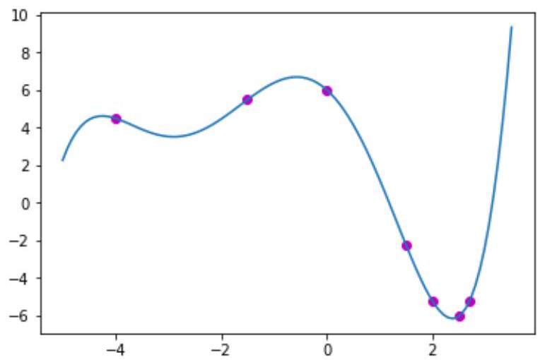
              
Fig. 7.8 gives the true solution (curve) and training data (dots).
Figure 7.8: True solution and training data for Gaussian Process example
The mean vector and covariance matrix can be generated for this problem using the following code.
# Kernel
              def kernel(X1,X2):
                # Sigma = np.exp(-(X1.reshape(X1.shape[0],-1) - X2)**2/2)
                Sigma = np.empty((X1.shape[0],X2.shape[0]))
                for i in range(X1.shape[0]):
                    for j in range(X2.shape[0]):
                        Sigma[i,j] = np.exp(-(X1[i]-X2[j])**2/2)
                return Sigma
              def mean(X):
                Mu = np.zeros(X.shape[0]) #np.mean(X,axis=0)
                return Mu
              Sigma = kernel(X_train,X_train)
              Mu = mean(X_train)
              
The following is not a necessary step for problem-solving. We just want to see what we will get from multivariate Gaussian sampling without relating the training data to the testing data (Fig. 7.9).
# Sampling for showing the Gaussian samples
              Sigma_sampling = kernel(X_true,X_true)
              Mu_sampling = mean(X_true)
              
for n_sampling in range(10):
                Y_sample = np.random.multivariate_normal(Mu_sampling,Sigma_sampling) #with smoothing (Sigma with
                    kernel)
                plt.figure(2)
                plt.plot(X_true,y_sample)
                Y_sample = np.random.multivariate_normal(Mu_sampling,np.eye(Mu_sampling.shape[0])) #without
                    smoothing (Sigma without kernel)
                plt.figure(0)
                plt.plot(X_true,y_sample)
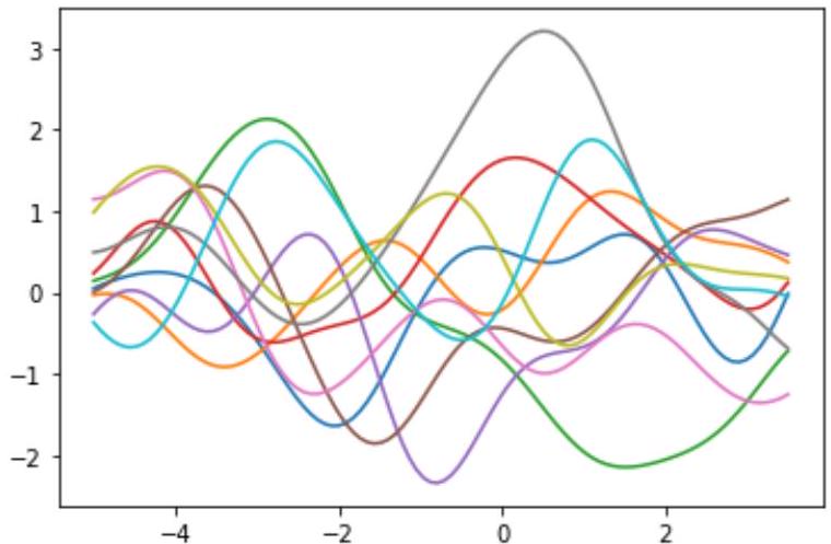
              
Figure 7.9: Multivariate Gaussian sampling without relating training data to testing data
The next step is the key step for conditioning multivariate Gaussian, which will obtain the coefficients for the testing data.
# Prediction
              X_pred = X_true
              K_whole = kernel(np.hstack((X_train,X_pred)),np.hstack((X_train,X_pred))) # Sigma matrix for the
                combined Gaussian distribution of [X_train, X_pred]
              K = K_whole[0:X_train.shape[0],0:X_train.shape[0]]
              K_ast = K_whole[:X_train.shape[0],X_train.shape[0]:]
              K_ast_ast = K_whole[X_train.shape[0]:,X_train.shape[0]:]
              M = Mu
              M_ast = mean (X_pred)
              Mu_pred = M_ast + ( K_ast.T @ np.linalg.inv(K) @ (y_train - Mu).reshape((y_train.size,1)) ).reshape(
                M_ast.size)
              Sigma_pred = K__ast_ast - K_ast.T @ np.linalg.inv(K) @ K_ast
              
With the GP model, we can then sample ten curves and plot the result.
plt.figure(3)
              for n_sampling_pred in range(10):
                y_pred = np.random.multivariate_normal(Mu_pred,Sigma_pred)
                plt.plot(X_pred,y_pred) # Plot n (number of iterations) predicted curves
              
Finally, we can obtain the average curve and confidence intervals by assessing the curves that we sample.
plt.plot(X_pred,Mu_pred) # Predict average prediction
              # sigma = np.std(X_pred) # Incorrect
              sigma = Sigma_pred.diagonal()**0.5 # Correct
              plt.fill_between(X_pred,Mu_pred-2*sigma,Mu_pred+2*sigma,color='yellow',alpha=0.9) # Show the region
                with mu +- sigma (68%) (2*sigma is 95%, 3*sigma is 99.7%)
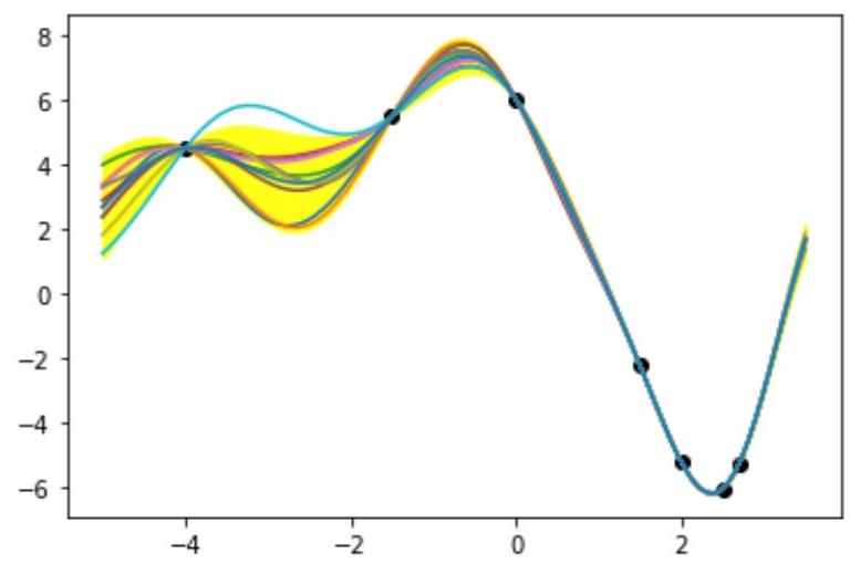
              
The final results are shown in Fig. 7.10.

Summary

After going through the above theory and implementation, we can draw the following key points about Gaussian process.
Figure 7.10: Final results of Gaussian Process analysis
  1. At each point for prediction, which can be viewed as the points for interpolation, the prediction at this point is treated as a random variable whose value can be drawn from a multivariate Gaussian distribution.
  2. One set of predicted target values at all the prediction data points represents one possibility from the multivariate Gaussian distribution.
  3. The average curve of all the predicted curves is the mean (most possible) prediction. The ranges of different confidence can also be obtained. Thus, GP does not give out one definite prediction, but instead, gives out different sets of predictions (corresponding to different models) that correspond to different probabilities.
  4. Prediction at different points (including the training points) in a set of predictions (one curve) are related to each other via the kernel function in the covariance matrix of multivariate Gaussian. This kernel function, which can use different math functions, is given to define how to smoothen the curve; Usually, the closer the prediction point is to a training point, the smaller the difference in their target values.
  5. The training points form a multivariate Gauss distribution with the prediction points. Thus, their values determine the general trends and means of predictions at the neighboring prediction points.
    Besides, please note that the selection of the kernel is made by human experts while the determination of the parameters can be done automatically by minimizing a loss term. This is the realm of Gaussian process regression. Finally, the handling of noisy data also deserves close attention, especially when we cannot get perfect samples of the hidden function. In this case, we need to factor this uncertainty into the model for better generalization.
In summary, the locations (X_train) and target values (y_train) of the training points, the selection of the kernel function, and the locations of the prediction data points (X_pred) determine what the predictions look like. The predictions are different curves with different probabilities.


Enjoy and Build the AI World

Sample Code from AI Engineering

Cite the code in your publications

Linear Models